How to Combine Debit and Credit Columns into One Amount Column (Excel and Power Query)
Turn separate debit and credit (paid out / paid in) columns into one signed amount with an Excel formula or Power Query, including fixes for text numbers.
Many banks export money out and money in as two separate columns — Debit and Credit, Paid out and Paid in, or Withdrawals and Deposits. QuickBooks Online's 3-column import, Xero's statement import and most analysis in Excel or Power BI need a single signed amount: negative for money out, positive for money in. This guide shows three ways to get there, from a one-line formula to a reusable Power Query step.
The goal
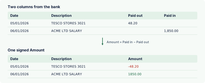
Here's a typical export and the result we want:
| Date | Description | Paid out | Paid in | → Amount |
|---|---|---|---|---|
| 05/01/2026 | TESCO STORES 3021 | 48.20 | -48.20 | |
| 06/01/2026 | ACME LTD SALARY | 1,850.00 | 1850.00 | |
| 08/01/2026 | OCTOPUS ENERGY | 75.00 | -75.00 |
Why one signed column is better
QuickBooks Online will accept separate columns in its 4-column layout, so why combine them? Three reasons. A single signed amount is what Xero's statement import and most accounting apps expect. It makes totals trivial: one SUM gives the net change for the period, which you can check against the statement in seconds. And in Power BI or a pivot table, one numeric column with a clear sign is far easier to work with than two half-empty ones — measures such as money in, money out and net movement become simple filters on the same column rather than separate calculations that have to be kept in step.
Method 1: An Excel formula
With Paid out in column C and Paid in in column D, add a new column and enter:
=N(D2)-N(C2)
Fill it down. N() turns an empty cell into 0, so the formula works whichever column is filled. Money in comes out positive and money out negative.
If your bank already puts a minus sign on debits (some do, showing -48.20 in the Paid out column), use ABS so the sign isn't flipped twice:
=ABS(N(D2))-ABS(N(C2))
When the numbers are stored as text
If the formula returns 0 for every row, the amounts are text rather than numbers — common when a CSV includes currency symbols, thousands separators or trailing spaces. You'll usually see them left-aligned in the cell. Clean them inside the formula:
=IFERROR(VALUE(SUBSTITUTE(SUBSTITUTE(D2,"£",""),",","")),0)-IFERROR(VALUE(SUBSTITUTE(SUBSTITUTE(C2,"£",""),",","")),0)
Replace "£" with "$" or your own currency symbol. Once the new column looks right, copy it and use Paste Special → Values so it no longer depends on the original columns, then delete Paid out and Paid in.
Method 2: One amount column plus a Dr/Cr column
Some banks give one positive amount plus a separate column that says whether it's a debit or a credit — DR/CR, D/C or Debit/Credit:
| Date | Description | Amount | Type |
|---|---|---|---|
| 05/01/2026 | TESCO STORES 3021 | 48.20 | DR |
| 06/01/2026 | ACME LTD SALARY | 1850.00 | CR |
With the amount in C and the type in D:
=IF(LEFT(UPPER(TRIM(D2)),1)="D",-ABS(C2),ABS(C2))
This treats anything starting with D (DR, D, Debit) as money out and everything else as money in.
Method 3: Power Query (repeatable)
If you clean the same bank's export every month, Power Query saves you from redoing the formulas. In Excel, select the data and choose Data → From Table/Range; in Power BI, load the CSV with Get data. Then open Advanced Editor and add a step like this after your source step (here called Source):
Clean = Table.TransformColumns(Source, {
    {"Paid out", each try Number.From(Text.Remove(Text.From(_), {"£", "$", ",", " "})) otherwise null, type nullable number},
    {"Paid in",  each try Number.From(Text.Remove(Text.From(_), {"£", "$", ",", " "})) otherwise null, type nullable number}
}),
WithAmount = Table.AddColumn(Clean, "Amount",
    each (if [Paid in] = null then 0 else Number.Abs([Paid in]))
       - (if [Paid out] = null then 0 else Number.Abs([Paid out])),
    type number),
Result = Table.RemoveColumns(WithAmount, {"Paid out", "Paid in"})
Each step goes inside the query's let block, separated by commas, and the last line of the query should read in Result. Change the column names to match your bank's export. The try … otherwise null part means blank or odd cells become empty instead of stopping the refresh with an error. Next month, replace the source file and select Refresh.
A note on dates in Power Query
If the dates come through wrong, it's the locale, not the data. Right-click the date column and choose Change Type → Using Locale…, then pick Date and the locale that matches the bank — English (United Kingdom) for day-first dates, English (United States) for month-first. See bank formats by country for which is which.
In Google Sheets
The same formulas work in Google Sheets. To fill a whole column at once without dragging, put this in the first data row of an empty column, with Paid out in C and Paid in in D:
=ARRAYFORMULA(IF(A2:A="", "", N(D2:D) - N(C2:C)))
If the amounts were imported as text, use VALUE(REGEXREPLACE(TO_TEXT(D2:D), "[^0-9.]", "")) in place of N(D2:D) — but note that this also strips minus signs, so only use it on columns that hold positive numbers. Wrap it in IFERROR(…, 0) to turn blanks into zeros.
Common mistakes
- Flipping the sign twice. If the Paid out column already shows
-48.20, subtracting it gives+48.20. UseABSas shown in Method 1. - Treating the balance column as an amount. Running balances are numbers too. Only combine the two transaction columns.
- Losing decimals with regional settings. A file that uses commas for decimals (
48,20) is read as 4820 by an English-language Excel. Use Data → Text to Columns → Advanced to set the decimal separator, or import with the right locale in Power Query. - Forgetting the summary rows. Some exports end with a Total line. Delete it before adding up, or the totals check will be out by exactly the total.
Check the result

Before you import, prove nothing was lost. Three quick checks:
- Totals: the sum of the negative amounts should equal minus the total of the Paid out column, and the sum of the positive amounts should equal the total of Paid in. Use
=SUMIF(E:E,"<0")and=SUMIF(E:E,">0"). - Count: the number of non-zero amounts should equal the number of transactions on the statement.
- Balance: opening balance + the sum of the Amount column should equal the closing balance.
If a row has both a debit and a credit filled in, the formula nets them. That's rare in bank exports, but check for it with =COUNTIFS(C:C,"<>",D:D,"<>") — it should return 1 (just the header row).
Or let a converter do it
If the end goal is QuickBooks or Xero, our QuickBooks converter and Xero converter detect separate debit and credit columns automatically and produce a single signed amount, plus the right column layout and date format for the import. They run in your browser, so the file isn't uploaded.
Checklist
- Money in is positive and money out is negative.
- Text amounts (with £, $, commas or spaces) were converted to numbers.
- Debits that already had a minus sign weren't flipped twice.
- Totals in and out still match the original columns.
- The formula column was pasted as values before deleting the originals.
- Dates were checked for the right day/month order.